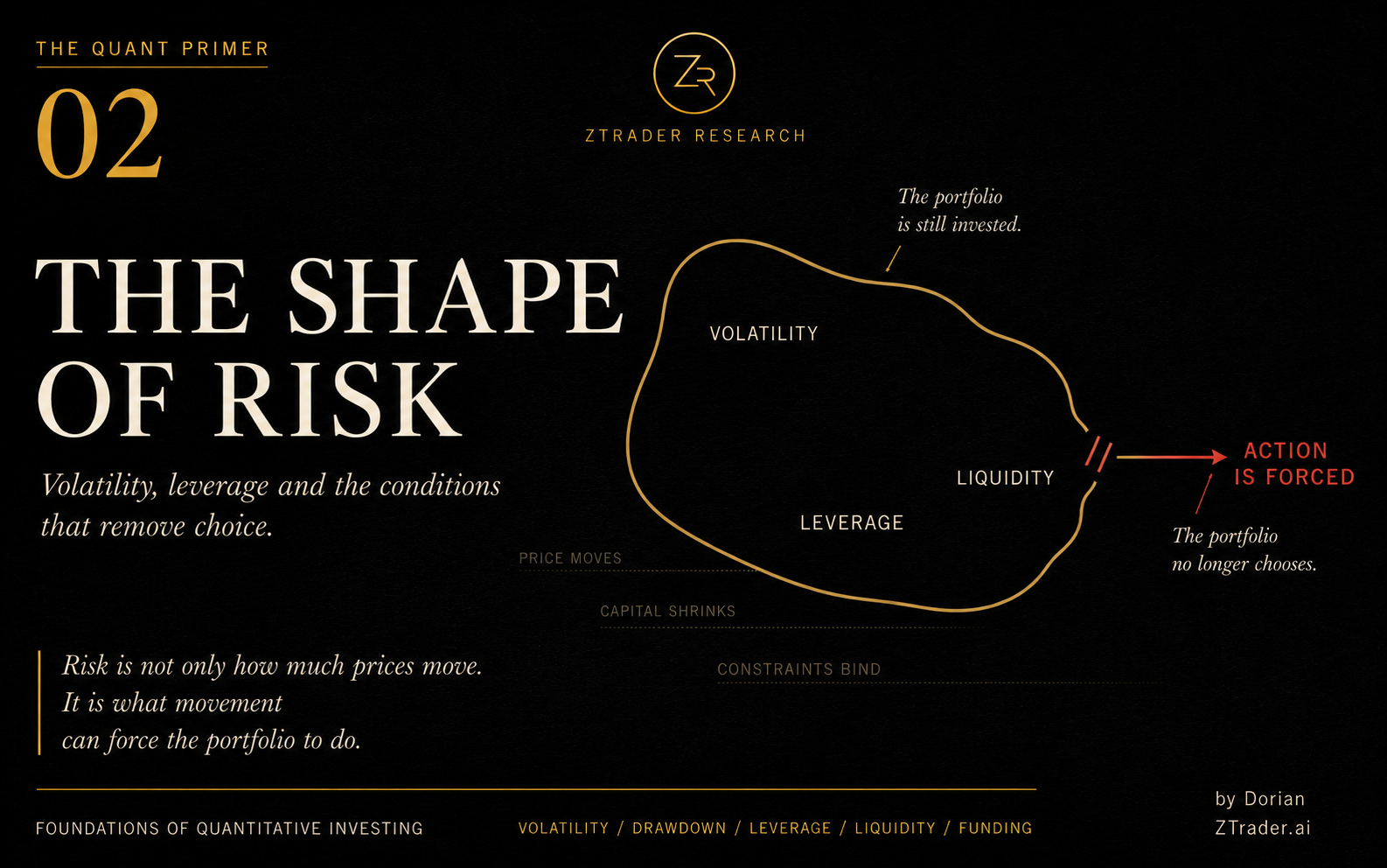

Volatility, leverage and the conditions that remove choice.
Risk becomes easier to manage after it has been converted into a common unit.
A portfolio runs at twelve percent volatility. A position contributes forty basis points of daily value-at-risk. A systematic strategy targets a ten percent annualized standard deviation. Figures like these allow exposures with different prices, histories and market conventions to enter the same risk budget. Without that compression, a multi-asset portfolio would quickly dissolve into intuition and incompatible units.
The convenience comes with a temptation. Once a precise estimate appears on a screen, it begins to look like an explanation of the portfolio rather than a description of one feature of its recent behavior.
Volatility measures the dispersion of returns. Capital encounters a more complicated object. A loss can arrive gradually in a deep market, leaving enough time to reduce exposure without changing the thesis. The same measured loss can arrive after a long period of calm, just as leverage is high, liquidity retreats and financing becomes more restrictive. Both episodes contribute observations to a volatility estimate. Only one may remove the investor's ability to wait.
Price movement matters, but the economic damage depends on the conditions surrounding it.
Volatility remains indispensable. It simply cannot answer a question it was never designed to answer:
Does the portfolio still control what happens next?
What the number contains
Historical volatility is an estimate built from choices that disappear inside the final decimal.
A sixty-day window gives recent observations more influence than a five-year sample. Exponentially weighted models react quickly to new information but can also reduce exposure after much of the move has already occurred. Daily closes ignore intraday instability, while higher-frequency data introduces its own distortions through bid-ask bounce, stale prices and market microstructure.
None of this makes the estimate arbitrary. It means the estimate is conditional on the history selected and the method used to summarize it.
Portfolio construction adds another layer. A volatility-targeting strategy usually scales exposure inversely to estimated risk:
Here, σ* is the desired volatility, σ̂t is the current estimate and k captures the remaining constraints of the portfolio.
The arithmetic is straightforward. If estimated volatility falls, the permitted position grows. If the estimate doubles, exposure is reduced by roughly half. That response can stabilize realized portfolio risk, provided the estimate continues to describe the conditions under which the position can be traded.
Moreira and Muir found that volatility-managed portfolios produced higher Sharpe ratios across several equity factors and currency carry in their sample. Their result did not rely on the idea that high volatility automatically predicts negative returns. The more important observation was that factor volatility varied substantially over time, while expected returns did not rise enough during volatile periods to compensate investors for maintaining constant exposure.
The research gives volatility management a serious empirical foundation. It does not settle the question that matters before leverage is increased. A low estimate may reflect durable stability, or it may simply describe an interval during which the forces capable of producing a discontinuity have remained inactive.
The formula can identify calm. It cannot determine what the calm is storing.
Calm can become an input into leverage
A quiet market alters more than the number printed beside "risk."
Lower realized volatility expands the amount of exposure that many institutions are permitted to hold. Stable collateral supports more borrowing. Narrower spreads make leveraged trades appear easier to finance and easier to exit. Rising prices improve measured balance-sheet strength, which can open additional capacity just as the market begins to look least threatening.
Each adjustment can be defensible on its own. The problem appears through their interaction.
Suppose a risk-parity portfolio observes declining covariance across its major exposures. The model permits more notional risk. A relative-value fund sees the same calm through tighter financing spreads and increases gross leverage. Dealers, facing stable collateral and subdued market movement, become more willing to intermediate. None of these participants needs to believe that the market has become permanently safe. Their constraints merely translate the same environment into larger balance sheets.
The Committee on the Global Financial System has examined this procyclical relationship between market-sensitive valuations, leverage and funding liquidity. During favorable periods, rising prices and declining measured risk encourage expansion. Once the direction reverses, weaker valuations and more restrictive financing force balance sheets to contract.
The market may therefore look stable partly because institutions have adapted their portfolios to stability. As long as the regime persists, the adaptation reinforces the appearance of calm. Prices remain orderly, spreads stay narrow and historical risk estimates decline further.
The vulnerability is not hidden in one particular model. It lies in the fact that many different models can produce the same balance-sheet response.
When the condition supporting those positions changes, the market does not begin from a neutral state. It begins with exposure already sized for a world that has just ended.
Returns arrive in an order
A distribution treats returns as observations. A portfolio receives them as a sequence.
Consider two unlevered portfolios, each beginning with $100. Both experience one gain of twenty percent and one loss of twenty percent. The order does not affect the terminal value:
The four-dollar loss comes from compounding. A twenty percent decline requires a twenty-five percent recovery to return to the starting point.
Sequence becomes economically important once the portfolio is subject to constraints.
Portfolio A earns twenty percent first, reaching $120, then loses twenty percent and finishes at $96.
Portfolio B loses twenty percent first. Its lender responds by cutting the permitted exposure in half. The remaining capital participates in only half of the subsequent twenty percent recovery:
The market produced the same two returns. The financing structure transformed them into a different investment outcome.
The first loss did more than reduce the capital base. It changed the amount of the subsequent recovery the portfolio was allowed to own. A strategy that remained capable of recovering in statistical terms became incapable of recovering under the rules governing its balance sheet.
Drawdown begins to capture this reality more directly than variance because it records capital lost from a previous peak. Duration adds information that depth alone misses. A sharp decline followed by a rapid recovery imposes a different operating burden from an equally deep decline that leaves the portfolio below its high-water mark for several years. Redemptions, collateral calls and mandate limits do not wait for the long-run distribution to vindicate itself.
Neither drawdown nor duration predicts the future. Their value lies elsewhere: they preserve the fact that losses occur at a particular point in the life of the portfolio, when capital, obligations and financing capacity have particular values.
The route matters because the route can change the vehicle.
The real risk limit is forced action
Risk tolerance is often described as a psychological property.
A manager claims to be comfortable with a twenty percent drawdown. An investor says the mandate has a long horizon. A committee states that short-term volatility should not interfere with the strategy's long-run thesis.
These statements matter only while the structure allows them to matter.
A fund may be willing to tolerate a twenty percent decline, but that willingness becomes irrelevant if redemptions accelerate at ten percent, a prime broker changes margin requirements at twelve or an internal mandate forces de-risking at fifteen. The point at which the manager loses discretion may arrive long before the point at which the manager loses conviction.
Risk capacity is determined by the obligations surrounding the position: collateral agreements, funding terms, regulatory capital, redemption rights, liability schedules and the behavior of counterparties. These arrangements convert certain price movements into mandatory decisions.
Once that conversion occurs, the trade is no longer about where the asset should eventually be worth. The immediate question is what the balance sheet can survive before the thesis has time to play out.
Leverage makes the transition nonlinear. Borrowing magnifies the first decline, but the damage does not stop there. Lower equity supports less financing. Higher measured volatility can increase haircuts. Reduced funding forces sales, and those sales weaken the price of the collateral supporting the remaining position. A market view gradually becomes a balance-sheet event.
The meaningful risk limit is therefore not the distance to an arbitrary stop-loss. It is the distance to the first condition capable of making the next action compulsory.

Liquidity belongs inside the position
A portfolio is valued using current market prices. Risk calculations then tend to assume that exposure can be changed somewhere near those marks.
The assumption is most credible before the portfolio needs to test it.
Market liquidity refers to the ability to trade without causing a large price concession. Funding liquidity refers to the ability to obtain or retain the financing required to continue holding the position. The two are often modeled separately, even though stress can bind them together.
Brunnermeier and Pedersen showed how worsening market liquidity can increase funding pressure, while constrained funding reduces traders' capacity to provide liquidity. Higher margins may amplify the decline because investors must sell more collateral into a market already losing depth. What begins as a change in price can develop into a feedback loop between balance sheets and transaction costs.
A stop-loss does not remove this mechanism. It identifies a level at which the portfolio would prefer to exit. It says nothing about the price available once many holders reach comparable limits. During stress, the stop becomes an instruction to compete for liquidity with every other institution trying to conserve cash.
The US Treasury market in March 2020 offered an unusually clear example. Leveraged relative-value investors faced margin and funding pressure as relationships that had normally moved within narrow ranges widened sharply. Forced deleveraging collided with limited dealer balance-sheet capacity, contributing to severe dysfunction in a market typically treated as one of the deepest and safest in the world.
The episode matters because it separates quoted liquidity from available liquidity. A security can trade in enormous volume under ordinary conditions and still become difficult to exit at scale once the same balance sheets are required to absorb the same direction of flow.
Liquidity is not an attribute permanently stored inside an asset. It is a service supplied by other participants, under terms they are free to revise when the environment becomes least convenient for the owner of the position.
Correlation can become a funding relationship
Diversification relies on the idea that different positions respond to different economic forces.
Historical covariance provides a practical way to estimate those relationships. In normal markets, the method can identify meaningful offsets among equities, rates, currencies and credit. The difficulty emerges when stress introduces a common factor that was not visible in ordinary return behavior.
An equity index, a currency carry trade and a credit position may be economically distinct. They can still be financed by the same intermediaries, held by funds operating under comparable risk constraints or sold through the same limited pool of dealer capacity. Once those investors need cash, growth, inflation and valuation may cease to organize the portfolio. Liquidation becomes the dominant factor.
The resulting correlation is not mysterious. Assets fall together because the same owners must reduce gross exposure, the same collateral agreements become restrictive and the same markets provide the easiest route to cash.
Currency carry offers a useful example. Brunnermeier, Nagel and Pedersen documented negative skew in carry-trade returns and linked crashes to abrupt unwinds during periods of deteriorating funding liquidity and risk appetite. The return premium existed during ordinary conditions, but the loss mechanism became visible when similar positions were forced through the same exit.
A correlation matrix estimated in calm markets may therefore describe the sample accurately while missing the relationship that matters during deleveraging. The diversification was real at the level of historical price behavior. The concentration existed at the level of ownership and financing.
Portfolio diversification should be tested in both languages. One asks whether returns have moved together. The other asks whether the positions can be forced to move together.
Smooth returns may be deferred liabilities
Some strategies earn a premium because they accept losses that arrive infrequently.
Insurance makes the structure obvious. Premium income is collected continuously, while claims arrive irregularly. A month without a claim does not create free alpha. It records income earned while the associated liability remained dormant.
Financial markets contain many versions of the same trade.
Short-volatility strategies collect option premium while remaining exposed to discontinuous movement. Credit earns spread while bearing default and liquidity risk. Carry strategies receive yield differentials while retaining vulnerability to funding shocks and crowded unwinds. Relative-value trades harvest small pricing discrepancies while relying on leverage, convergence and uninterrupted financing.
These strategies can appear unusually efficient during ordinary periods because the income arrives gradually and the loss does not. Hit rates remain high. Recent volatility stays low. Drawdowns appear manageable until the event that justifies the premium finally occurs.
The mistake is not accepting an asymmetric payoff. An investor may rationally sell insurance, own credit or run carry when the compensation is adequate and the tail exposure is understood.
The mistake appears when the premium is separated from the liability that produced it.
Stable returns are then treated as evidence that the strategy has discovered an unusually clean source of alpha, even though the portfolio has merely postponed the moment when its obligation becomes visible.
A useful analysis should identify what the strategy is underwriting. Without that answer, smoothness can become a form of accounting camouflage.
Risk control has an execution price
A volatility-targeting rule reduces exposure when estimated risk rises. In a model, the adjustment happens at the observed price and requires no negotiation.
The market is less cooperative.
Suppose a portfolio targets ten percent volatility and the estimate rises from ten to twenty percent. Holding the other inputs constant, permitted exposure falls by half. The model has not formed a bearish view. The existing position has simply become too large for the mandate.
If liquidity remains available, the portfolio may resize without disrupting the strategy. Under stress, the transaction occurs under less forgiving conditions. Spreads widen, market depth declines and other investors may be reacting to similar constraints. The portfolio must reduce risk by demanding liquidity at the moment liquidity has become scarce.
March 2020 showed the broader mechanism without requiring volatility-targeting funds to be the original cause. Rising volatility, margin pressure, leverage reduction and constrained intermediation interacted across Treasury and funding markets. The shock became more damaging because balance sheets had to adjust while the market's capacity to absorb those adjustments was deteriorating.
This distinction matters. Volatility management can improve long-run portfolio behavior, as the Moreira and Muir evidence suggests. The technique does not fail merely because it reduces exposure after volatility rises. The vulnerability lies in assuming that the necessary trade can always be executed at the price embedded in the risk model.
Every reduction in exposure has timing, capacity and market impact.
Risk control is therefore not outside execution. It is one of the most consequential executions the portfolio will ever make.

Models fail at their boundaries
Unexpected losses often produce a familiar response: improve the distribution.
Use fatter tails. Shorten the volatility window. Raise the confidence level. Make correlations more responsive. Increase the frequency of stress tests.
Any of these changes may improve the estimate. None can guarantee that the structure surrounding the estimate remains intact.
A model can calculate correctly while the assumptions governing execution and financing deteriorate. The quoted spread may not support the required order size. Financing may no longer be available on historical terms. Several hedges may depend on the same dealer balance sheet. Positions that appeared diversified may reveal a shared liquidation channel.
Moving value-at-risk from a 95 percent to a 99 percent confidence level introduces a more conservative statistical threshold. It does not make a discontinuous market continuous. It does not ensure that collateral can still be financed or that an exit remains available after every crowded portfolio reaches the same constraint.
A risk estimate should therefore be read as a conditional statement:
Given these assumptions about returns, liquidity, financing and market behavior, the portfolio is expected to behave within these bounds with the stated frequency.
The important questions concern the assumptions carrying the most weight. Which ones are likely to fail together? How quickly would the portfolio detect the failure? Which position would need to be sold first? Who else would be using the same exit?
The model describes the portfolio inside an operating environment. Risk management must also examine the operating environment.
A portfolio needs several risk languages
No single measure can describe every way a portfolio can fail.
Volatility estimates the ordinary scale of return variation, but it does not distinguish continuous movement from discontinuity. Drawdown records the amount of capital already lost from a previous peak, while duration reveals how long the portfolio has remained impaired. Skew and tail measures expose asymmetry, though their estimates remain dependent on the history available.
Leverage determines how quickly an asset loss reaches equity. Liquidity determines the concession required to change the position. Funding determines whether the portfolio is allowed to keep holding it. Stress tests explore combinations that may not have appeared in the sample, and concentration analysis looks beyond security names to identify shared economic theses, counterparties and exit routes.
The goal is not to place every statistic on one enormous dashboard. A dense display can hide weak reasoning just as effectively as a single volatility number. The useful distinction is whether each measure answers a different operating question.
A credible risk process should be able to explain:
what causes the portfolio to lose;
what can make the loss accelerate;
which constraint is capable of forcing action;
and what remains tradable once action is required.
Volatility informs those questions by describing the scale and variability of movement. The remaining answers come from the structure around the trade.

Conclusion
Volatility remains essential because it gives heterogeneous positions a common language. It helps determine exposure, combine assets and impose discipline on portfolios that would otherwise be governed by intuition.
The danger begins when the common language is mistaken for a complete description of the system.
Portfolios do not fail because a standard deviation becomes morally unacceptable. They fail when price movement reaches leverage, when collateral terms change, when financing becomes conditional or when several positions discover that they depend on the same liquidity.
A patient strategy can survive a volatile market if it retains capital, funding and the ability to trade. A statistically conservative strategy can fail in a quieter market if its structure allows a modest move to trigger mandatory liquidation.
The critical distinction is therefore not between calm and volatility.
It is between a portfolio that can still choose
and one whose next decision has already been made for it.
Research Anchors
- Moreira, Alan; Muir, Tyler. Volatility-Managed Portfolios. NBER Working Paper No. 22208; subsequently published in The Journal of Finance.
- Brunnermeier, Markus K.; Pedersen, Lasse Heje. Market Liquidity and Funding Liquidity. NBER Working Paper No. 12939; subsequently published in The Review of Financial Studies.
- Brunnermeier, Markus K.; Nagel, Stefan; Pedersen, Lasse Heje. Carry Trades and Currency Crashes. NBER Working Paper No. 14473.
- Committee on the Global Financial System. The Role of Valuation and Leverage in Procyclicality. CGFS Papers No. 34, Bank for International Settlements.
- Schrimpf, Andreas; Shin, Hyun Song; Sushko, Vladyslav. Leverage and Margin Spirals in Fixed Income Markets During the Covid-19 Crisis. BIS Bulletin No. 2.
- Avalos, Fernando; Ehlers, Torsten; Eren, Egemen. BIS research on leverage, margining and vulnerabilities in US Treasury futures.